class: center, middle, inverse, title-slide # Unsupervised Analysis ## JHU Data Science ### www.jtleek.com/advdatasci --- class: inverse, middle, center # Final Project Discussion --- class: inverse ## In approximate order of difficulty .super[ * Descriptive <br><br> * Exploratory <br><br> * Inferential <br><br> * Predictive <br><br> * Causal <br><br> * Mechanistic <br><br> * Unsupervised/Supervised ] --- class: inverse ## Supervised vs. unsupervised .super[ Supervised * You have an outcome YY and some covariates XX <br><br> * You typically want to solve something like `\(\arg\min_{f} E[(Y−f(X))^2]\)` Unsupervised * You have a bunch of observations X and you want to understand the relationships between them. <br><br> * You are usually trying to understand patterns in X or group the variables in X in some way ] --- class: inverse background-image: url(../imgs/unsupervised/face.png) background-size: 35% background-position: center # Semi-supervised .footnote[http://static.googleusercontent.com/media/research.google.com/en/us/archive/unsupervised_icml2012.pdf] --- class: inverse ## A few techniques for unsupervised .super[ * Kernel density estimation <br><br> * Clustering <br><br> * Principal components analysis/SVD <br><br> * Factor analysis <br><br> * MDS/ICA/MFPCA/... ] --- class: inverse ## Example: stamp thickness ```r library(bootstrap) str(stamp) ``` ``` 'data.frame': 485 obs. of 1 variable: $ Thickness: num 0.06 0.064 0.064 0.065 0.066 0.068 0.069 0.069 0.069 0.069 ... ``` ```r thick = stamp$Thickness head(stamp) ``` ``` Thickness 1 0.060 2 0.064 3 0.064 4 0.065 5 0.066 6 0.068 ``` --- class: inverse ## Summary statistics .left-column-equal[ ```r ggplot(stamp, aes(y = Thickness, x = 1)) + geom_boxplot(outlier.shape = NA) + geom_jitter(height = 0) + theme_big ``` <!-- --> ] .right-column-equal[ ```r boxplot(thick); stripchart(thick, add =TRUE, vertical=TRUE, jitter=0.1, method = "jitter", pch=19, col=2) ``` <!-- --> ] --- class: inverse background-image: url(../imgs/unsupervised/binning.png) background-size: 70% background-position: bottom # Binning --- class: inverse ## You've seen this: histograms ```r par(mfrow=c(1,2)) hist(thick,col=2); hist(thick,breaks=100,col=2) ``` <!-- --> --- class: inverse background-image: url(../imgs/unsupervised/est_density.png) background-size: 80% background-position: bottom # Estimating the density --- class: inverse background-image: url(../imgs/unsupervised/kde.png) background-size: 60% background-position: bottom # Kernel density estimator --- class: inverse ## You've seen this, too .left-column-equal[ ```r ggplot(stamp, aes(x = Thickness)) + geom_density() ``` <!-- --> ] .right-column-equal[ ```r dens = density(thick); plot(dens, col=2) ``` 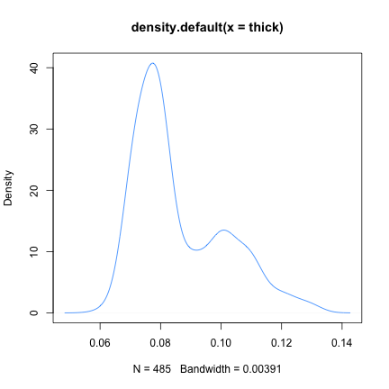<!-- --> ] --- class: inverse ## Make our own kde ```r normer = function(x) dnorm(dens$x, mean=x, sd=dens$bw)/length(thick) plot(dens$x, normer(thick[1]), type="l") for(i in 1:length(thick)){ lines(dens$x, normer(thick[i]), col=2) } ``` 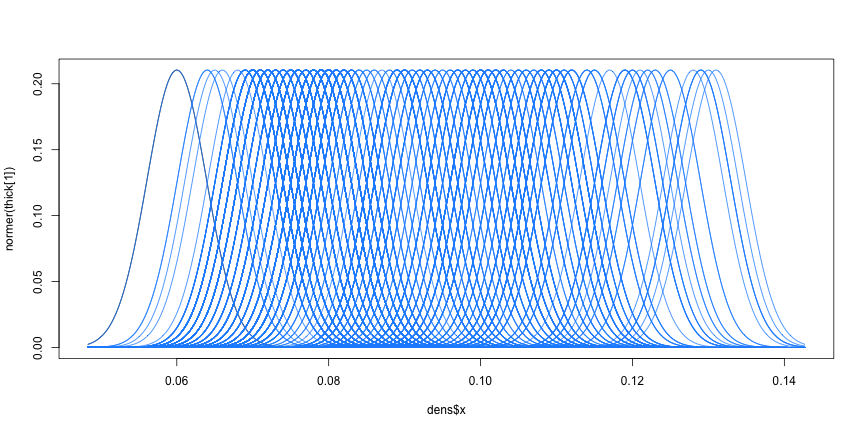<!-- --> --- class: inverse ## Make our own kde ```r dvals = rep(0,length(dens$x)) for(i in 1:length(thick)){ dvals = dvals + dnorm(dens$x,mean=thick[i],sd=dens$bw)/length(thick) } plot(dens,col=3,lwd=3); points(dens$x,dvals,col=2,pch=19,cex=0.5) ``` 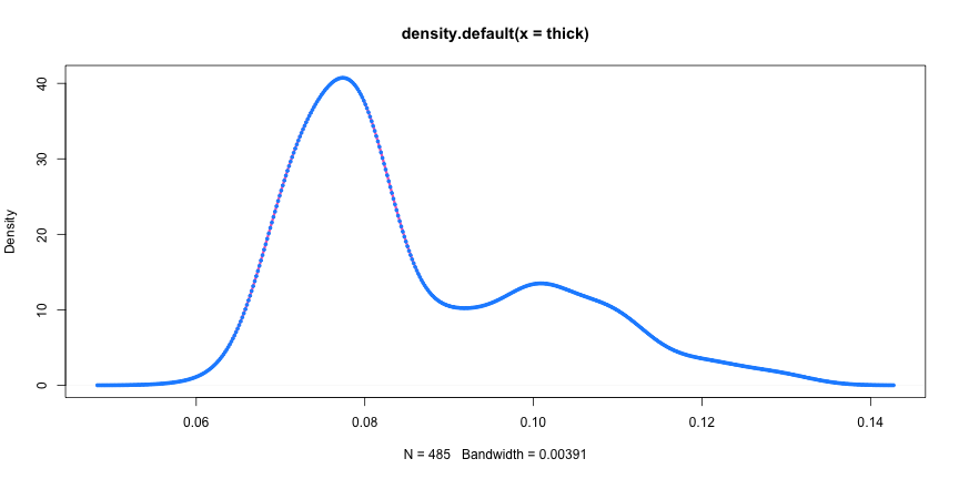<!-- --> --- class: inverse, middle, center # Exercise: How would we estimate the number of modes in a density estimate as a function of hh? --- class: inverse ## One answer .super[ ```r nmodes <- function(y) { x <- diff(y) n <- length(x) sum(x[2:n] < 0 & x[1:(n - 1)] > 0) } nmodes(dens$y) ``` ``` [1] 2 ``` ] --- class: inverse background-image: url(../imgs/unsupervised/smooth_ex.png) background-size: 25% background-position: center # Smoothing example .footnote[http://genomicsclass.github.io/book/] --- class: inverse ## Smoothing example ```r library(Biobase); library(SpikeIn); library(hgu95acdf); data(SpikeIn95) ##Example with two columns i = 10; j = 9 ##remove the spiked in genes and take random sample siNames <- colnames(pData(SpikeIn95)) ind <- which(!probeNames(SpikeIn95) %in% siNames) pms <- pm(SpikeIn95)[ind , c(i, j)] ##pick a representative sample for A and order A Y = log2(pms[, 1]) - log2(pms[, 2]) X = (log2(pms[, 1]) + log2(pms[, 2])) / 2 set.seed(4) ind <- tapply(seq(along = X), round(X * 5), function(i) { if (length(i) > 20) { return(sample(i, 20)) } else { return(NULL) } }) ind <- unlist(ind); X <- X[ind]; Y <- Y[ind] o <- order(X); X <- X[o]; Y <- Y[o] ``` --- class: inverse ## Smoothing example ```r fit <- lm(Y ~ X); plot(X, Y); points(X, Y, pch = 21, bg = ifelse(Y > fit$fitted, 1, 3)) abline(fit, col = 2, lwd = 4, lty = 2) ``` 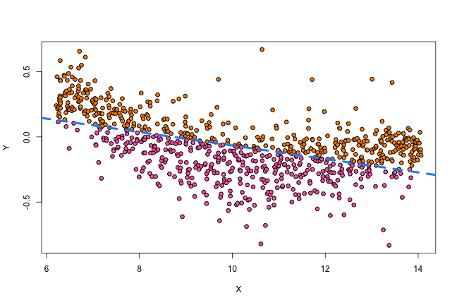<!-- --> --- class: inverse ## Bin smoothing ```r centers <- seq(min(X), max(X), 0.1) windowSize <- 1.25 i <- 25 center <- centers[i] ind = which(X > center - windowSize & X < center + windowSize) fit <- lm(Y ~ X, subset = ind) ``` --- class: inverse ## Bin smoothing ```r plot(X, Y, col = "darkgrey", pch = 16); points(X[ind], Y[ind], bg = 3, pch = 21) a <- min(X[ind]); b <- max(X[ind]) lines(c(a, b), fit$coef[1] + fit$coef[2] * c(a, b), col = 2, lty = 2, lwd = 3) ``` <!-- --> --- class: inverse ## Many windows ```r windowSize <- 0.5 smooth <- rep(NA, length(centers)) for (i in seq(along = centers)) { center <- centers[i] ind = which(X > center - windowSize & X < center + windowSize) smooth[i] <- mean(Y[ind]) if (i %% round(length(centers) / 12) == 1) { ##we show 12 plot(X, Y, col = "grey", pch = 16) points(X[ind], Y[ind], bg = 3, pch = 21) lines(c(min(X[ind]), max(X[ind])), c(smooth[i], smooth[i]), col = 2, lwd = 2) lines(centers[1:i], smooth[1:i], col = "black") points(centers[i], smooth[i], col = "black", pch = 16, cex = 1.5) } } ``` <!-- --><!-- --><!-- --><!-- --><!-- --><!-- --><!-- --><!-- --><!-- --><!-- --><!-- --><!-- --> --- class: inverse ## The result ```r par(mfrow=c(1,1)) plot(X,Y,col="darkgrey",pch=16) lines(centers,smooth,col=2,lwd=3) ``` <!-- --> --- class: inverse ## Loess .left-column-equal[ ```r i <- 25; center <- centers[i]; ind = which(X > center - windowSize & X < center + windowSize) fit <- lm(Y ~ X, subset = ind) ``` <!-- --> ] .right-column-equal[ ```r i <- 60 center <- centers[i] ``` <!-- --> ] --- class: inverse ## Final result for loess ```r fit <- loess(Y ~ X, degree = 1, span = 1 / 3) newx <- seq(min(X), max(X), len = 100) smooth <- predict(fit, newdata = data.frame(X = newx)) plot(X, Y, col = "darkgrey", pch = 16); lines(newx, smooth, col = "black", lwd = 3) ``` <!-- --> --- class: inverse background-image: url(../imgs/unsupervised/loess.png) background-size: 50% background-position: center # A big deal! .footnote[http://amstat.tandfonline.com/doi/abs/10.1080/01621459.1979.10481038 ] --- class: inverse background-image: url(../imgs/unsupervised/curse_dimensionality.png) background-size: 65% background-position: bottom # Curse of dimensionality --- class: inverse ## Clustering - when you have many variables .huge[ Clustering organizes things that are <font color="yellow">close</font> into groups * How do we define close? * How do we group things? * How do we visualize the grouping? * How do we interpret the grouping? ] --- class: inverse background-image: url(../imgs/unsupervised/cluster_analysis.png) background-size: 60% background-position: center # Another big one! .footnote[https://scholar.google.com/scholar?hl=en&q=cluster+analysis&btnG=] --- class: inverse background-image: url(../imgs/unsupervised/distance.png) background-size: 50% background-position: center # Defining close .footnote[http://rafalab.jhsph.edu/688/lec/lecture5-clustering.pdf] --- class: inverse background-image: url(../imgs/unsupervised/euclid.png) background-size: 60% background-position: center # Euclidean distance --- class: inverse background-image: url(../imgs/unsupervised/manhattan.png) background-size: 50% background-position: center # Manhattan distance .footnote[http://en.wikipedia.org/wiki/Taxicab_geometry] --- class: inverse ## Hierarchical clustering .left-column-equal[ <img src = "../imgs/unsupervised/hierarchical.png" style="width:80%"> ] .right-column-equal[ .super[ An agglomerative approach * Find closest two things * Put them together * Find next closest Requires * A defined distance * A merging approach Produces * A tree showing how close things are to each other ] ] --- class: inverse, center ## Hierarchical clustering - an example 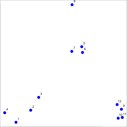<!-- --> --- class: inverse ## Distances ```r dataFrame <- data.frame(x = x, y = y); pheatmap(dist(dataFrame), cluster_rows = FALSE, cluster_cols = FALSE) ``` 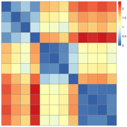<!-- --> --- class: inverse ## Step one - find closest ```r library(fields); dataFrame <- data.frame(x = x, y = y) rdistxy <- rdist(dataFrame); diag(rdistxy) <- diag(rdistxy) + 1e5 ind <- which(rdistxy == min(rdistxy), arr.ind = TRUE) ``` 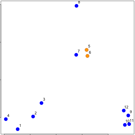<!-- --> --- class: inverse ## Step one - find closest ```r distxy = dist(dataFrame); hcluster = hclust(distxy) dendro = as.dendrogram(hcluster); cutDendro = cut(dendro,h=(hcluster$height[1]+0.00001) ) ``` 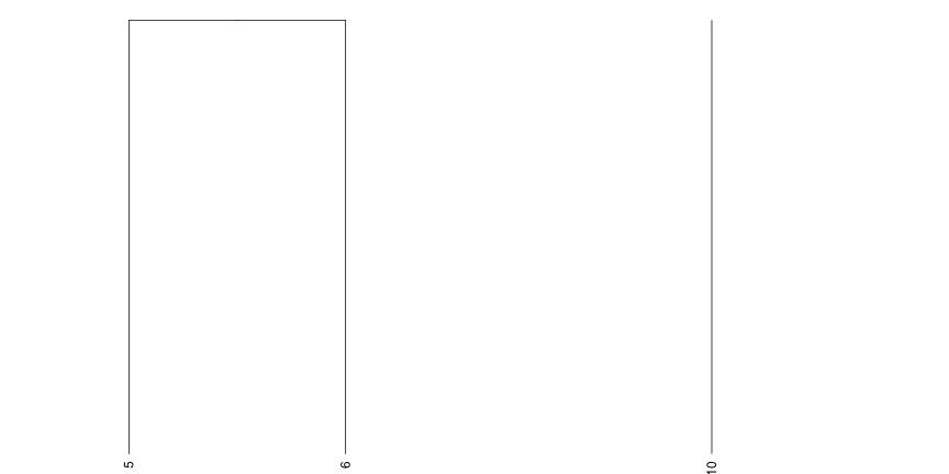<!-- --> --- class: inverse ## Step two - merge closest 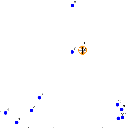<!-- --> --- class: inverse ## Find next closest and repeat ```r ind <- which(rdistxy == rdistxy[order(rdistxy)][3], arr.ind = TRUE) ``` 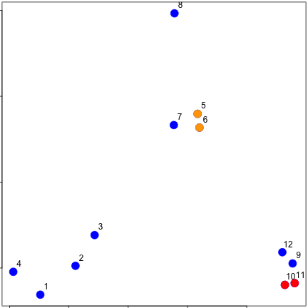<!-- --> --- class: inverse ## Find next closest and repeat ```r cutDendro <- cut(dendro, h = (hcluster$height[2])) ``` 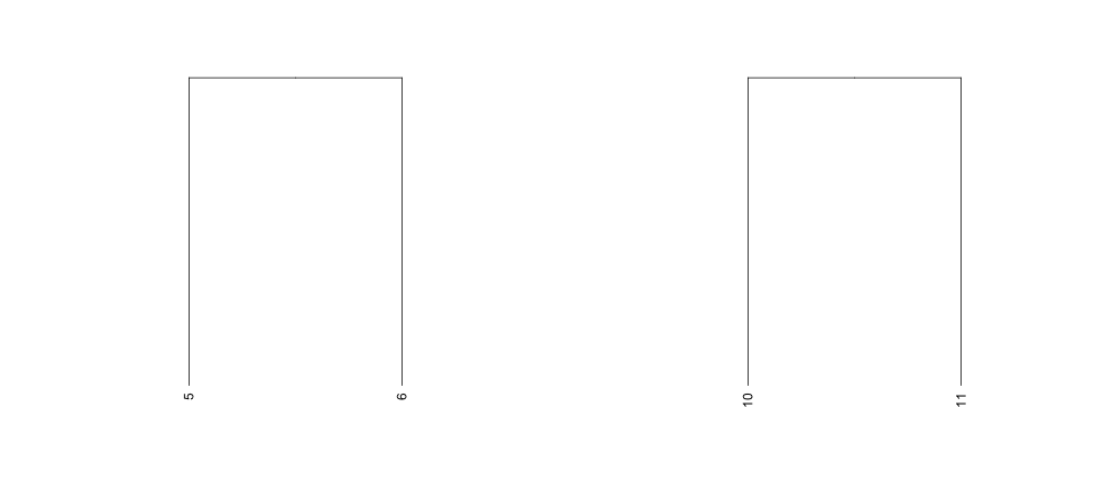<!-- --> --- class: inverse ## Hierachical clustering - hclust ```r dataFrame <- data.frame(x=x,y=y); distxy <- dist(dataFrame); hClustering <- hclust(distxy) ``` 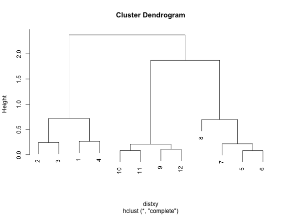<!-- --> --- class: inverse background-image: url(../imgs/unsupervised/merging.png) background-size: 40% background-position: center # Merging points - complete --- class: inverse background-image: url(../imgs/unsupervised/merging_avg.png) background-size: 40% background-position: center # Merging points - average --- class: inverse background-image: url(../imgs/unsupervised/linkage.png) background-size: 70% background-position: bottom # What these choices look like --- class: inverse ## K-means clustering .left-column-equal[ <img src = "../imgs/unsupervised/kmeans.png" style="width:100%"> ] .right-column-equal[ .super[ A partioning approach * Fix a number of clusters * Get "centroids" of each cluster * Assign things to closest centroid * Reclaculate centroids Requires * A defined distance metric * A number of clusters * An initial guess as to cluster centroids Produces * Final estimate of cluster centroids * An assignment of each point to clusters ] ] --- class: inverse ## K-means example ```r x = rnorm(12, mean = rep(1:3, each = 4), sd = 0.2) y = rnorm(12, mean = rep(c(1, 2, 1), each = 4), sd = 0.2) ``` 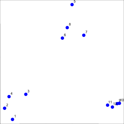<!-- --> --- class: inverse ## K-means - starting centroids ```r cx <- c(1,1.8,2.5); cy <- c(2,1,1.5) ``` 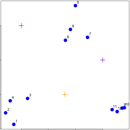<!-- --> --- class: inverse ## K-means - assign to closest centroid ```r distTmp <- matrix(NA,nrow=3,ncol=12); d = function(i) (x-cx[i])^2 + (y-cy[i])^2; distTmp[1,] <- d(1); distTmp[2,] <- d(2); distTmp[3,] <- d(3); newClust <- apply(distTmp,2,which.min); points(x,y,pch=19,cex=2,col=cols1[newClust]) ``` 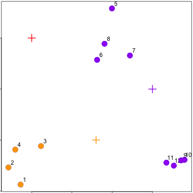<!-- --> <!-- ***MISSING SLIDES HERE*** --> --- class: inverse ## K-means ```r dataFrame <- data.frame(x,y) kmeansObj <- kmeans(dataFrame,centers=3) names(kmeansObj) ``` ``` [1] "cluster" "centers" "totss" "withinss" [5] "tot.withinss" "betweenss" "size" "iter" [9] "ifault" ``` ```r kmeansObj$cluster ``` ``` [1] 1 1 1 1 2 2 2 2 3 3 3 3 ``` --- class: inverse background-image: url(../imgs/unsupervised/model_based.png) background-size: 70% background-position: bottom # Model based clustering --- class: inverse background-image: url(../imgs/unsupervised/em.png) background-size: 50% background-position: bottom # Estimating parameters - EM like approach --- class: inverse background-image: url(../imgs/unsupervised/bayes.png) background-size: 80% background-position: center # Select the number of clusters with Bayes factors --- class: inverse background-image: url(../imgs/unsupervised/faithful.png) background-size: 40% background-position: center # Old faithful example .footnote[https://en.wikipedia.org/wiki/Old_Faithful] --- class: inverse ## Update ```r library(mclust); faithfulMclust <- Mclust(faithful) summary(faithfulMclust,parameters=TRUE) ``` ``` ---------------------------------------------------- Gaussian finite mixture model fitted by EM algorithm ---------------------------------------------------- Mclust EEE (ellipsoidal, equal volume, shape and orientation) model with 3 components: log.likelihood n df BIC ICL -1126.361 272 11 -2314.386 -2360.865 Clustering table: 1 2 3 130 97 45 Mixing probabilities: 1 2 3 0.4632682 0.3564512 0.1802806 Means: [,1] [,2] [,3] eruptions 4.475059 2.037798 3.817687 waiting 80.890383 54.493272 77.650757 Variances: [,,1] eruptions waiting eruptions 0.07734049 0.4757779 waiting 0.47577787 33.7403885 [,,2] eruptions waiting eruptions 0.07734049 0.4757779 waiting 0.47577787 33.7403885 [,,3] eruptions waiting eruptions 0.07734049 0.4757779 waiting 0.47577787 33.7403885 ``` --- class: inverse ## Update ```r plot(faithfulMclust) ``` 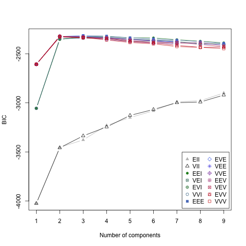<!-- --><!-- --><!-- --><!-- --> --- class: inverse ## A pathological example ```r clust1 = data.frame(x=rnorm(100),y=rnorm(100)); a = runif(100,0,2*pi) clust2 = data.frame(x=8*cos(a) + rnorm(100),y=8*sin(a) + rnorm(100)) plot(clust2,col='blue',pch=19); points(clust1,col='green',pch=19) ``` <!-- --> --- class: inverse ## What happens ```r dat = rbind(clust1,clust2); kk = kmeans(dat,centers=2); plot(dat,col=(kk$clust+2),pch=19) ``` 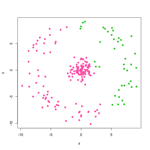<!-- --> --- class: inverse ## Clustering wrap-up .super[ * Algomerative (h-clustering) versus divisive (k-means) <br><br> * Distance matters! * Merging matters! <br><br> * Number of clusters is rarely estimated in advance <br><br> * H-clustering: Deterministic - but you don’t get a fixed number of clusters <br><br> * K-means: Stochastic - fix the number of clusters in advance <br><br> * Model based: Can select the number of clusters, may be stochastic, careful about assumptions! ]