14 Week 13
14.1 Week 13 Learning objectives
At the end of this lesson you will be able to:
- Define the set of expected outcomes for an analytic system
- Define a data analytic anomaly
- Describe the process of debugging a data analysis
- Identify root causes of data analytic anomalies
14.2 Introduction
Lucky Week 13 has arrived! And perhaps fittingly, we will discuss the process of what to do when things go wrong.
The presentation of how data analyses are conducted is typically done in a forward manner. A question is posed, data are collected, and given the question and data, a system of statistical methods is assembled to produce evidence. That evidence is then interpreted in the context of the original question. While such a description provides a useful model, it is incomplete in that it assumes the statistical methods are completely determined by the question and the data. In practice, there is an equally important “backwards” process that data analysts use to either revise their statistical approach or investigate potential problems with the data. This process of revision is driven by observing deviations between the data and what we expect the data to look like.
Much previous work dedicated to studying the data analysis process has focused on the notion of “statistical thinking,” or the cognitive processes that occur within the analyst while doing data analysis. Grolemund and Wickham refer to these “forwards” and “backwards” aspects of data analysis as part of a sense-making process, where analysts attempt to reconcile schema that describe the world with data that are measured from the world. Should there be a discrepancy between the schema and the data, the analyst can update the schema to better match the observed data. These updates ultimately result in knowledge being accumulated.
14.3 Basic Data Analytic Iteration
In the course of any data analysis, at some point we are confronted with a basic activity, which can be called the basic data analytic iteration. This iteration is at the core of the sense-making process described by Grolemund nad Wickham. The iteration only begins once we look at some data. At that point, we must decide to do something (or do nothing). Once we make that decision, the iteration begins anew. In the course of executing this iteration, we may observe something that is unexpected, and that is what this lecture is about. These unexpected outcomes are what we will call anomalies.
Characterizing anomalies in data analysis requires that we have a thorough understanding of the entire system of statistical methods that are being applied to a given dataset. Included in this system are traditional statistical tools such as linear regression or hypothesis tests, as well as methods for reading data from their raw source, pre-processing, feature extraction, post-processing, and any final visualization tools that are applied to the model output. Ultimately, anomalies can be caused by any component of the system, not just the statistical model, and it is the data scientist’s job to understand the behavior of the entire system. Yet, there is little in the statistical literature that considers the complexity of such systems and how they might behave under real-world conditions.
Once we have set off with a scientific question (even if vaguely stated), we can go on to collecting or assembling some data to address that question. Typically, we will need to build and develop develop a system of statistical methods that we can apply to the data to generate evidence. This system includes every aspect of contact with the data, including reading the data from its source, pre-processing, modeling, visualization, and generation of output.
The basic data analytic iteration comes in four parts. Once a question has been established and a plan for obtaining or collecting data is available, we can do the following:
- Construct a set of expected outcomes
- Apply a data analytic system to the data
- Diagnose any anomalies in the analytic system output
- Make a decision about what to do next
In this lecture, we are going to focus on the first three steps of this iteration, and in particular, Step 3. But first, we need to talk about statistical methods systems and the set of expected outcomes.
14.4 Statistical Methods Systems
To study the manner in which data analyses can produced unexpected results, it is useful to first consider data analyses as a system of connected components that produce specific outputs. A statistical methods system is a collection of data analytic elements, procedures, and tools that are connected together to produce a data analysis output, such as a plot, summary statistic, parameter estimate, or other statistical quantity. By connecting these elements and tools together, we create a complex system through which data are transformed, summarized, visualized, and modeled. Each of the components in the system will have its own inputs and outputs and tracing the path of those intermediate results plays a key role in developing an understanding of the system.
There are also contextual inputs to the data analysis, such as the main question or problem being addressed, the data, the choice of programming language to use, the audience, and the document or container for the analysis, such as Jupyter or R Notebooks. While these inputs are not necessarily decided or fundamentally modified by the analyst, the data analyst may be expected to provide feedback on some of these inputs. In particular, should an analysis produce an unexpected result, the analyst might identify one of these contextual inputs as the root cause of the problem.
A statistical methods system can be characterized as a sequence of steps or a deterministic algorithm. The algorithm is not necessarily uni-directional and may double-back on itself and branch into multiple sections. Ultimately, the algorithm produces an output that may be interpreted by the analyst or passed on to serve as input to another system. In describing the behavior of any system, one must be careful to define the resolution of the system (i.e. how detailed we want to specify steps) and the boundaries of the system diagram. In particular, we should acknowledge what elements are excluded from the diagram, such as application-specific context or other assumptions. The development of a statistical methods system would typically be guided by statistical theory, as well as knowledge of the scientific question, any relevant context or previous research, available resources, and any design requirements for the system output.
14.4.1 Example: A Simple Linear Model System
Consider a system that fits a simple linear model as part of a data analysis. This system reads in some data on a pair of variables \(x\) and \(y\), fits a simple linear regression via least squares, and outputs the intercept and slope estimates. A depiction of this system along with some representative R code is shown in Figure 1.
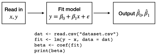
Simple linear regression statistical methods system with pseudo-code.
The diagram indicates that understanding how this system operates
requires knowledge of (1) how the data are read in; (2) how the model is
fit to the data; and (3) how the estimated coefficients are extracted
from the model fit and outputted. Specifically, if we are using R to
analyze the data, we must have an understanding of the read.csv(),
lm(), coef(), and print() functions.
14.5 The Set of Expected Outcomes
Once a statistical methods system is built, but before it is applied to the data, we can develop a set of expected outcomes for the system. These expected outcomes represent our current state of scientific knowledge and may reflect any gaps or biases in our understanding of the data, the problem at hand, or the behavior of the statistical methods system. The overarching goal of the data analysis is to produce outputs that will in some way improve our understanding of the scientific problem. Without any expected outcomes, it is challenging to interpret the output of the system or determine how the output informs our understanding of the underlying data generation process.
An important property of the set of expected outcomes is that the expected outcomes are always stated in terms of the observed output of the system, not any underlying unobserved population parameters. We draw a distinction here between hypotheses, which are statements about the underlying population, and expected outcomes, which are statements about the observed sample data. Another property of the set of expected outcomes is that they will generally have sharp boundaries. Therefore, once we observe the output from the statistical methods system, we know immediately and with complete certainty whether the output is expected or unexpected (i.e falls into the set or not). Boundaries of this nature are important for the analyst so that decisions can be made regarding any next steps in the analysis.
Developing a useful set of expected outcomes is part of the design process for a statistical methods system and depends on many factors, including our knowledge and assumptions about the underlying data generation process, our ability to model that process using statistical tools, our knowledge of the theoretical properties of those tools, and our understanding of the uncertainty or variability of the observed data across multiple samples. Hence, even though the underlying truth might be thought of as fixed, it is reasonable to assume that different analysts might develop different sets of expected outcomes, reflecting differing levels of familiarity with the various factors involved and different biases towards existing evidence or data.
14.5.1 Example: Expected Outcomes for the Sample Mean
In some contexts, the set of expected outcomes may be derived from formal statistical hypotheses. For example, we may design a system to compute the sample mean \(\bar{x}\) of a dataset \(x_1,\dots,x_n\) that we model as being sampled independently from a \(\mathcal{N}(\mu,1)\) distribution. In this case, the output from the system is \(\bar{x}\) and based on our current knowledge we may hypothesize that \(\mu=0\). Under that hypothesis, we might expect \(\bar{x}\) to fall between \(-2/\sqrt{n}\) and \(2/\sqrt{n}\). For \(n=10\), this interval is \([-0.63,0.63]\) and any observed value of \(\bar{x}\) outside that interval would be an anomaly.
Another analyst might be more familiar with this data generation process and therefore hypothesize that the underlying population mean is \(\mu=3\) without assuming a Normal distribution. This analyst might also know that the data collection process can be problematic, leading to very large outlier observations on occasion. Therefore, based on experience and intuition, this analyst has a wider expected outcome interval of \([1, 5]\).
In both examples here, the set of expected outcomes was a statement about \(\bar{x}\), the output of the system applied to the observed data. The set of expected outcomes was also a fixed interval with clear boundaries, making it straightforward to determine whether the output would fall in the interval or not.
14.6 Anomaly Space
An anomaly occurs only if there is a clearly defined set of expected outcomes for a system, and the observed output from the system does not fall into that set. The specification of an anomaly then requires three separate elements:
A description of what specific system output or collection of outputs is observed;
A description of how the outputs deviate from their expected outcomes; and
An indication of when or under what conditions the deviation is observed.
Continuing the example from the previous section, an anomaly for the sample mean could be “\(\bar{x}\) is outside the expected interval of \([-0.63, 0.63]\) when a sample of size \(n=10\) is inputted to the system”. The observed output is \(\bar{x}\), the deviation is "outside the interval \([-0.63, 0.63]\)", and the event occurs when \(n=10\).
The anomaly space of a statistical methods system consists of the collection of potential outputs from the system which would indicate that an anomaly has occurred. Fundamentally, the anomaly space is the complement of the set of expected outcomes. Not all areas of the anomaly space are equally important and in some applications it may be that anomalies occuring in certain subsets of the anomaly space are more interesting than anomalies occurring elsewhere. The size of the anomaly space of a statistical methods system is determined by the outputs produced by the system. Looking back to the simple linear model system in Figure 1, there are only two outputs (\(\hat{\beta}_0\) and \(\hat{\beta}_1\)) that define the anomaly space. Therefore, any anomalies for that system must be determined by those two values.
As the number of system outputs grows, the size of the anomaly space may grow accordingly. For example, we can increase the size of the anomaly space for the simple linear model system by also returning the standard errors of the coefficients. With each additional output, we increase the number of ways in which anomalies can occur. Different systems with different sets of outputs will induce anomaly spaces of differing sizes and the nature of the anomaly space associated with a system may serve as a factor in choosing between systems. Also, because the anomaly space depends on the specification of the set of expected outcomes, different analysts with different expectations could induce different anomaly spaces for the same statistical methods system.
Once a statistical methods system has been applied to the data and an anomaly has been observed, the “forward” aspect of data analysis is complete and the analyst must begin the “backward” aspect to determine what if any changes should be made to the analysis. Such changes could involve modifying the statistical methods system itself or could require changes to our set of expected outcomes based on this new information. However, before any decision can be made in response to observing an anomaly, a data analyst must enumerate the possible root causes of the anomaly and determine which root causes should be investigated.
14.7 Debugging Anomalies
Once a statistical methods system has been applied to a dataset and the output is observed, we can determine whether an anomaly has occurred based on our understanding of the set of expected outcomes. If an anomaly occurs, we must attempt to identify its root cause. To do so, we can use the following process:
State the anomaly in terms of what output, how it deviates, and when it is observed to occur.
Reconstruct the entire sequence events (or as much as possible based on available information) that occurs leading up to the anomaly. This can be a sequence of code statements or a more abstract system diagram. The reconstruction can be detailed or not depending on how much information is available. With a reproducible analysis, it should be possible to reconstruct all the steps.
Starting with the output, trace back through the system diagram or sequence of code statements and enumerate any possible sources of error and their likelihood of occurring. This process may branch off in different directions at each stage of the system diagram/code.
Stop the process once we either reach an explanation that lies outside the system or we have identified a set of root causes that is not worth developing any further.
Summarize the root causes.
Once you’ve made your best efforts to identify the root causes of an anomaly, you must then decide what to do. We will not go into detail here about that decision process, but typically, you will want to follow up further on any key root causes. For example, if it’s possible that there is a problem with the data collection process, you might want to follow up with the people who originally collected the data to find out more information.
14.7.1 Basic Example
Consider the basic system shown below.
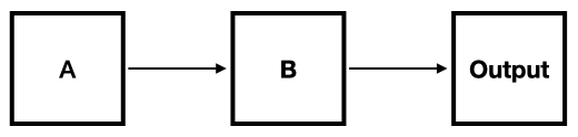
Basic System Diagram
If we observe an anomaly in the “Output” portion of the sytem, we can trace backwards through the system to identify possible causes. In this process it is important to take a very myopic and step-by-step approach to ensure that we do not skip over anything (i.e. “think small”).
In the figure above, if there is a problem with the “Output” then that problem might have originated in component “B”, which generates the output. So the first cause might be
- Bad output from “B”
Moving back further, we might say either
- Good input to “B”, but bad output from “B”; or
- Bad input to “B”
The event 2 above represents a failure of component “B”, which probably should be investigated. However, event 3 suggests there is a problem with component “A”.
Here, the root causes are either
- A problem with component “B” even when the input is good
- A problem with component “A”
Given the simplicity of the system diagram in this example, it’s not surprising that the set of root causes is small.
Depending on the complexity of the system diagram, the debugging process could get similarly complicated. One possible way to simplify things is to break the system down into sub-systems in order to compartmentalize the different (independent) aspects of the system.
14.7.2 Example: Debugging a Simple Linear Model System
We can describe the process of debugging the simple linear model system shown below.
Simple linear regression statistical methods system with pseudo-code.
Let’s say, for example, that under normal operation, we might expect that \(\hat{\beta}_1\approx 2\). With typical random variation in the data we might expect \(\hat{\beta}_1\) to range from 0 to about 4. Therefore, based on past experience, it would be highly unexpected to observe \(\hat{\beta}_1<0\) or \(\hat{\beta}_1>4\). For this example, we will define the anomaly of interest as
\(\hat{\beta}_1 < 0\) when printed to the console.
Note that although the set of expected outcomes is the interval \([0, 4]\), we define the anomaly as \(\hat{\beta}_1<0\) and ignore the part of the anomaly space defined by \(\hat{\beta}_1>4\). Similarly, possible anomalies concerning the intercept \(\hat{\beta}_0\) will not be developed here.
Starting with the system description in the figure above, we can walk through the system backwards to identify any root causes. First, we might consider any problems with the print() function as it’s possible that the beta vector is fine but the print() function somehow corrupted it. This scenario is highly unlikely so we will then move backwards to the coef() function. Again, here, it’s unlikely thet coef() function is the cause of the problem as it’s very simple and has been in use a long time with linear models. This then brings us to the lm() function, which produces the model fit.
Should we observe \(\hat{\beta}_1<0\) there are perhaps two possibilities we might consider:
The structural relationship between \(x\) and \(y\) has changed to no longer reflect the simple linear model; or
The underlying structural relationship remains, but the input data to the linear model has been contaminated, perhaps with outliers.
The first case represents our expectations being incorrect, which is always a possibility. It is possible that we perhaps misunderstood the relationship between \(x\) and \(y\) in the first place. For example, it could be that the data are naturally more variable than we thought they were, and so our set of expected outcomes for \(\hat{\beta}_1\) should be much larger. In any case, any structural change also needs to be large enough (relative to the noise in the data) so that we are able to observe it in the data.
Developing the “contaminated data” event a bit further, we can propose that either there are outliers present in the raw data or outliers were somehow
introduced into the data before inputting to the regression model. Note the difference here: One version says there are contaminated data in the raw dataset that originates from outside the system. The other version says that the outliers were introduced somehow by reading the data in. This can happen if functions like read.csv() attempt to convert data from one format to another. Another possibility is that missing data are encoded in a special way (e.g. using -99 is common) that is unknown to the read.csv() function.
While the presence of outliers can be a root cause of the anomaly \(\hat{\beta}_1<0\), outliers do not always cause an unexpected change in \(\hat{\beta}_1\). The outliers also have to be arranged in such a manner that they cause \(\hat{\beta}_1\) to be \(< 0\), perhaps because of some selection process in the outlier generation/designation.
14.8 Summarizing Root Causes
Once a debugging analysis has been done to a statistical methods system regarding a particular anomaly we must summarize the root causes. In the simplie linear model example above, the root causes of the anomaly “\(\hat{\beta}_1<0\) when printed to the console” could be caused by
- A change in the structural relationship between \(x\) and \(y\) AND the change is large enough to be observed over the noise levels
- Contaminated observations in the raw data AND there is a selection process that arranges the contaminated data to produce \(\hat{\beta}_1<0\)
- Contamination is introduced in reading the data AND there is a selection process that arranges the contaminated data to produce \(\hat{\beta}_1<0\)
Once the set of root causes are identified, a decision must be made about what to do next. This decision will depend on a number of factors, including the likelihood of each root cause of occurring. For example, if it is highly likely that our model is wrong, we may not bother to investigate the possibility of contaminated data. However, if this is a process that we have worked with for a long time and are confident in the model, we may be more concerned with contamination in the data.
Another action we might take is to modify the system so that future applications to future datasets will provide more informative output. If it turns out that contaminated data can occasionally enter the system, we may want to introduce a step that filters those data, or perhaps stops the system when contaminated data are detected. Another possibility is to use a robust method that downweights extreme values.
Ultimately, making decisions about what to do in each cycle of a basic data analytic iteration depends on knowing the set of options. Debugging data analytic anomalies is about systematically generating a set of root causes so that the data scientist can choose what to investigate, what to ignore, and what to modify.
14.9 Homework
- Template Repo: https://github.com/advdatasci/homework13
- Repo Name: homework13-ind-yourgithubusername
- Pull Date: 2020/12/07 9:00AM Baltimore Time